NN primitives: Neurons to Transformers

Neural Networks have changed a lot since I first learnt about the simple DNNs back at school. How did we go from haha neurons go brrt to attention and memory and transformers?

So to help ME (and maybe you) better understand the foundations of modern ai, this is a brief primer written by yours truly to understand all the spanking new neural network primitives that have been developed.

Math and gory details are left as an exercise to the reader.

Primer Index

• Primitive Neurons and Pizza
• Multilayer Perceptrons, Backpropogation, and their families
• Sequential Data and RNNs
  • RNNs and memory
  • Training RNNs
• More memory primitives
  • LSTM Cells
  • Gated Recurrent Unit (GRU) cells
• Tokens and Embeddings
• Attention is all you need
  • Attention Functions
  • Transformer
• What next?

Primitive Neurons and Pizza

The death of humanity first began when we started to model our brains. The idea is simple. We model a neuron found in brains.

A neuron takes in a sum of weighted inputs, computes some function (step function), then outputs a value. The neuron here is called a Threshold Logic Unit, or TLU.

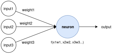
The math nerds are still arguing about what step function works best, but classically TLUs use a heaviside function (0 if input < 0 else 1) or sign function (-1 if input < 0 or 0 if input == 0 or 1 if input > 0).

With a TLU, the algorithm nerds found that it can do simple linear binary classification (1 for yes 0 for no).

From this primitive, we can build some nice stuff. We start with Perceptrons which is basically a layer of TLUs that takes in a bunch of inputs. For math reasons a bias neuron might be added to the input. This gives us a nice equation that I will definitely be using in my lifetime $h_{W,b}(X) = \phi(XW+b)$¹

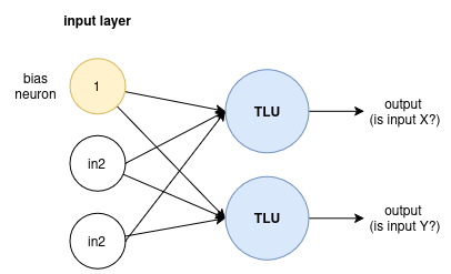
These perceptrons helped scientists answer the very pressing question of whether or not pizza is a soup, sandwich or salad.

Briefly, the perceptron learns whether X is a soup, sandwich or salad by running some training instances that we know the correct answer to. Based on the output, we adjust the weights to nudge the output neurons to give the correct answer if it predicts wrongly.

No one uses perceptrons these days anyway so I will leave the rule update specifics as a exercise for the reader, but just know that this NN model is limited in what patterns it can learn because the decision boundary is linear for each output neuron.

Multilayer Perceptrons, Backpropogation, and their families

Two nerds ranted that perceptrons suck cuz it cant solve some stupid linearly inseperable XOR problem. So they had the bright idea of throwing more neuron layers to the problem. And it works?

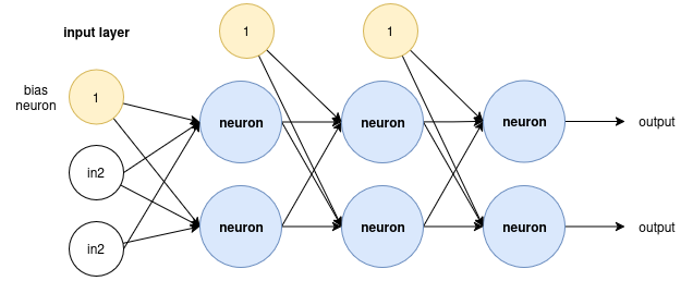
This is what most people are thinking of when it comes to NNs. We have lower layers (close to the input), hidden layers inbetween, and then upper layers close to the output layer.

Updating the weights is surprisingly hard (we have O(L*n^2) edges to update…). Unfortunately, some nerd came up with backpropogation. This algorithm is the bane of EE2211 victims (myself included), who have to manually run backprop during finals.

Buckle up and stop scrolling TikTok cuz alot of vocabulary ahead:

We divide our training set into mini-batches. We then throw it to the NN multiple times. Each pass is called an epoch.

FOR EACH MINI-BATCH, they are put into the NN in a forward pass, and we remember the intermediate results in each layer. We then check the output error (via some loss function).

Then we do math to see how much each output connection contributes to the error via chain rule. We repeat the chain rule for every layer, from upper to lower. This is a reverse pass, which computes the error gradient for all connection weights. We then do gradient descent to adjust all the weights, then move on to the next mini-batch.

Also important is to randomly init the weights, if not due to math the layers will behave as one neuron due to symmetry.

Btw the math nerds are still arguing about activation functions, so here’s a picture of commonly used ones from Kaggle and some stackexchange thread about when to use each one².

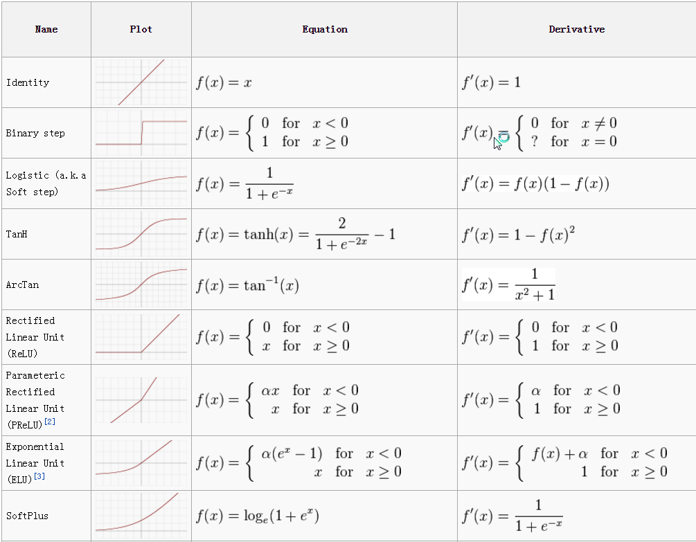
MLPs can be used for regression and classification tasks. Regression MLPs typically dont use any activation function for the output layer. For classification, we have as many output neurons as there are classes, and then we feed it to softmax function to give us multiclass probabilities.

Deep Neural Networks (DNN) are a superset of MLPs. MLPs are fully connected (between layers) DNNs. DNNs have minimally 1 hidden layer.

Convolutional Neural Networks (CNN) are special networks that are more specialized to deal with images/grid-like data best. They use pooling and convolution layers. The convolution layer applies kernels with weights to extract features. The pooling layer applies some mathematical function (avg, max, …) which shrinks the input size. See this stanford cheatsheet.

Speedrunning decades of research: We can do cool shit like reuse/fix pretrained gradients to not train from scratch. Optimizers are algorithms that are used to calculate gradients during backprop. Vanishing and exploding gradient issues are a thing, but are minimized with techniques like gradient clipping, Glorot initialization, and choosing other activation functions. Details are left as an exercise to the reader (i want to get to the more interesting bits…)

Sequential Data and RNNs

CNNs and DNNs are great for stateless problems. We don’t really care about the intermediate state of the input, such as images. But in comes the proto-hft nerd.

The proto-hft nerd wants to predict if Dogecoin will go to the moon. The proto-hft nerd has 365 days of dogecoin price data and a dream.

For this to work, the model needs to learn patterns that can appear over any arbitrary contiguous sequence of price points to accurately predict the next day’s price.

The nerd tries DNNs by flattening the data into a 365-dim input vector. This approach quickly falls apart. Structurally, the model does not inherently care about input order. The model also cannot share weights across positions. Patterns learned at one point of the window needs to be relearnt if it appears again³. And with larger datasets, the input vector scales.

The nerd tries CNNs, using a 1D conv with window of size 5 across the data. The model recognizes local patterns, but the pattern recognition is constrained by the kernel size. Some market patterns appear across a variety of window sizes, and CNNs cannot adapt.

This is where recurrent neural networks (RNN) come in, where it does well with sequential data as the architecture itself carries memory/state of the previous inputs of the sequence.

RNNs and memory

Our mental model of NNs gets a little bit more fucky wucky because we have to add one more dimension to the model. We extend the neuron’s state across time (or sequence).

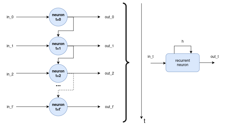
The recurrent neuron holds 2 sets of weights. One for inputs $x_t$ and the other for the outputs of the previous step $y_{t-1}$. We do some linear algebra magic that allows us to model the outputs of a layer to be some computable⁴ linalg equation. (HOML pg 499). $$ \begin{aligned} Y_t &= \phi(X_t W_x + Y_{t-1} W_y + b) \\ &= \phi\left( \begin{bmatrix} X_t & Y_{t-1} \end{bmatrix} W + b \right), \quad \text{where } W = \begin{bmatrix} W_x \ W_y \end{bmatrix} \end{aligned} $$

Since a recurrent neuron’s output at time t is a function of all the inputs from previous $t$. This recurrent neuron (cell) has some form of memory. A memory cell’s state at time $t$ is $h_t$. The hidden state, $h_t = f(h_{t-1}, x_t)$

A RNN can take in a sequence of inputs and produce a sequence of outputs, which can be used to predict how stock prices move over time. This is precisely when Jump River Street was born⁵.

Other useful cases apart from seq-to-seq are (Refer to HOML figure 15-4)…
Encoder: seq-to-vector networks where we only care about the last output of the sequence (sentiment analysis).
Decoder: vector-to-seq networks (asking chat to generate a caption for your image).
Encoder-Decoder: a combination of both (translation?)

Training RNNs

Training RNNs are not too different from classical DNNs. The idea is to unroll the memory cell through time, and then just run backpropagation. This is creatively named Backpropagation through time (BPPT).

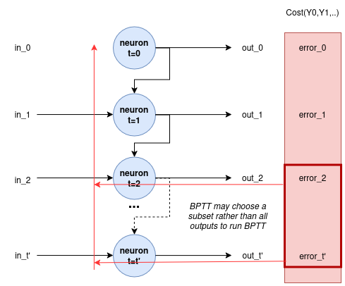
The idea is that BPTT can choose a subset of costs to run backprop on. The gradients flow through the appropriate output paths and all recurrent neuron states. Implementation details are usually abstracted from the user.

As always, we can stack recurrent cells and throw compute at the model and it will give us useful models.

More memory primitives

When data goes through the RNN, some information is lost at each time step. The RNN’s state will eventually reach a point where the initial input no longer has a trace in the RNN. Its like forgetting what you said earlier mid-sentence.

A few nerds improved on this goldfish memory problem by creating new cell architectures.

LSTM Cells

LSTM cells are better than recurrent neurons for remembering long term dependencies. Briefly, it takes in ‘cell’ long term state c, short term state h, as well as the input x. It outputs the current long term, short term, and output. Chain it together to get a LSTM layer.

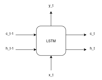
We now open up the LSTM box to be humbled. Because wtf is going on? This explainer is good.

The intuition behind LSTM is that we want the cell to be able to learn which long term states are worth retaining. It needs mechanisms to drop memories of previous states, and add memories of current states to remember.

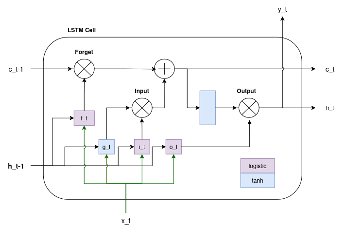
(x) here are element-wise multiplication, (+) is addition.

$g_t$ is the main layer. Similar to memory cells, it takes in short-term memory and the current input and stores it in long term memory.

$f_t, i_t, o_t$ are gate controllers. They control how open the gate should be. 1 for fully open, 0 for fully closed.

• $f_t$ => forget gate controls which long-term state should be erased
• $i_t$ => input gate controls which $g_t$ should be added to long term state
• $o_t$ => output gate controls which parts of the long-term state should be read and output (to y and short term memory) at the current timestep

All four functions defined above have learnable weights and biases, similar to the basic neurons. These equations make the cell easily computable.

$$ \begin{aligned} \begin{aligned} f_t &= \sigma(W_f [h_{t-1}, x_t] + b_f) \\ i_t &= \sigma(W_i [h_{t-1}, x_t] + b_i) \\ o_t &= \sigma(W_o [h_{t-1}, x_t] + b_o) \\ g_t &= \tanh(W_g [h_{t-1}, x_t] + b_g) \\ c_t &= f_t \odot c_{t-1} + i_t \odot g_t \\ y_t &= o_t \odot \tanh(c_t) \end{aligned} \end{aligned} $$

So, learning which memories to drop, retain, use, propagate are all learnable (trainable).

‘Peephole’ connections are an extension of LSTM. The long term memory c of the previous timestep is added to f, i gates; and the current long term state is also added to the connection of the output gate. The idea is that the long term memory can give more context to the cell. But the performance may or may not work (even the authors from the textbook im reading shrug it off)

Gated Recurrent Unit (GRU) cells

Some performance⁶ nerd decided to simplify the architecture of LSTM.

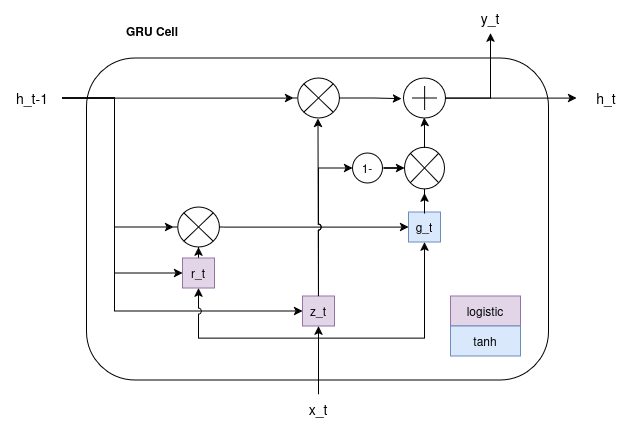
The idea: merge the long and short term state vectors into one (h). Control the forget and input gate via one gate controller $z$. The more the forget gate is open, the more the input gate is closed. We control how much the previous state is shown to the input layer $g$ by the gate controller $r$.

There are also linalg equations for GRU, but this will be left out for brevity.

Tokens and Embeddings

A few scientists were probably fans of Iron Man and wanted to make their own Jarvis. With the idea of memory, it’s entirely plausible that we could make a model that can mimick human language (since language is sequential data).

The problem is that RNNs need vectors. There needs to be a better way of modelling language.

Tokenizers are algorithms that break up natural language into tokens. See this tokenizer playground.

“The quick brown fox somersaulted over the lazy dog” could be tokenized into:

[“The”, “quick” “brown”, “fox”, “som”, “ers”, “ault”, “ed”, “over”, “the”, “lazy”, “dog”].

Tokenization converts raw text into sequence of discrete symbols from a finite vocabulary. (notice how somersaulted was split!)

The tokens are still not machine-readable. So we need to convert them into embeddings. Every token has a learned vector such that $E \in \R^{V \times d}$, where V is the vocab size and d is the embedding dimension.

Each token has a token id. We take the token id and fetch the corresponding embedding vector.

So a token like “the” can be converted to a d-dimension vector [0.91, -0.42, …, 0.76]. Each token can be sequentially funneled into the RNN. We can now build Jarvis.

It’s a good time to define what tensors are. Tensors are just a |col|-dimension representation of an object (token).

Our input to our spanking new neural network is an input tensor. Each row of the tensor corresponds to a token, and the columns are the representation space (how many features) of that token. This is a hyperparameter.

Attention is all you need

“Jarvis please take out the trash and then solve world hunger and also call Ms Penny to remind her of the upcoming corporate event at nine.”

This sentence is tokenized and fed into a RNN/LSTM/GRU. The trash was never taken out and the lab smells like sour fish the next day.

The issue is that when the network processes ‘upcoming’, information about ‘trash’ already travelled through many intermediate states. The model lost information about trash because there is only so much memory the model can hold.

To solve this problem, attention is all you need⁷.

Attention Functions

An attention mechanism looks back at the other tokens, computes its attention weights (importance) given a particular position.

Consider this example:

“The animal didn’t cross the road because it was tired”

The     0.01
animal  0.55 <- most relevant token  'it'
didn't  0.02
cross   0.03
the     0.01
road    0.08
because 0.04
it      0.05
was     0.08
tired   0.13

An attention function simply maps a query and a set of key-value pairs to an output. All the of the query, key, values are vectors. The output is typically a weighted sum of the values based on some compatability function.

Scaled Dot Product Attention

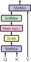
For a token i, we want an attention score for every token j via $q_i \cdot k_j$ and then scale by $\sqrt{d_k}$ to prevent vanishing gradients.

Represented in terms of linear algebra,

• Q query: what information am I looking for?
• K key: what information do I have?
• V value: what information do I provide?

$$ \text{Attention}(Q,K,V) = \text{softmax}(\frac{QK^T}{\sqrt{d_k}})V $$

Multi-head Attention

One attention score is not enough. It only captures one kind of relationship. We also want to introduce some way to ’learn’ via a weights matrix.

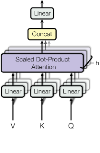
So, we run h (number of heads) independent attention operations in parallel.
Semantically this means want to learn h possible attention relationships.

We divide V, K, Q into $d_\text{model}/h$ size spaces each to make the math work out. Each subspace learns one relationship (learned projection). We then need to learn how to mix the learned relationships together with a final learned projection $W^O$.

In math-speak: $$ \begin{aligned} \text{MultiHead}(Q,K,V) &= \text{Concat}(h_1,h_2,\ldots,h_h)W^O \\ \text{where } h_i &= \text{Attention}(QW_i^Q,KW_i^K,VW_i^V) \end{aligned} $$

and

$$ W_i^Q \in \mathbb{R}^{d_{\text{model}}\times d_k} $$

$$ W_i^K \in \mathbb{R}^{d_{\text{model}}\times d_k} $$

$$ W_i^V \in \mathbb{R}^{d_{\text{model}}\times d_v} $$

$$ W^O \in \mathbb{R}^{hd_v\times d_{\text{model}}} $$

The output of multi-head attention is an enriched context-aware tensor. Recall that the rows represent the input token, and the columns represent the representation space of the token. The representation space is enriched with information from other tokens.

Positional encoding

Problem: The architecture of SDPA & MHA faces ordering problems similar to DNNs.

Because of math⁸ (permutation equivariance), we can shuffle around the order of input tokens (shuffling V, K, Q in the same way) and still get the same attention result for each token after applying Attention. Intuitively, consider “man eats chicken” and “chicken eats man”. After applying self-attention, ’eats’ will have the same attention score pointing to ‘man’ in both cases, although the semantics has changed (the attention score should be different to be correct).

The idea is to add information about a token’s position into a token’s embedding/vector. The information about a token’s position is positional encoding.

There are many ways of doing positional encoding, but the Transformer architecture uses a sinosoidal representation.

$i$ is the index over the dimension. Every even dimension is indexed over a sine curve with a unique frequency, and every odd dimension is indexeed over a cosine curve with unique frequency. Each dimension has it’s own sinusoidal function relative to position. Each position gets a ‘unique’ positional vector.

$$ PE_{(pos, 2i)} = \sin\left(\frac{pos}{10000^{2i/d_{\text{model}}}}\right) $$

$$ PE_{(pos, 2i+1)} = \cos\left(\frac{pos}{10000^{2i/d_{\text{model}}}}\right) $$

This encoding value is added to the vector of a given token. Since embeddings contain information about position, relationships learnt during multi-head attention are aware of position as well.

Add & Norm

Lastly, we have the feed forward network (FFN) and Add & Norm layers. FFNs are basically a DNN. Why do we have these two things?

Recall that the MHA generates a context-aware tensor. Information about the original tensor (prior to the attention block) is distorted due to mixing in of information from other tokens during the attention phase.

To prevent the initial tensor from being completely lost, and to prevent exploding magnitudes, we “Add and Normalise” the MHA tensor with the input tensor. This makes the attention tensor effectively an ‘update’. $X’ = X + \Delta X_\text{attention}$

Feed Forward Network

After add+norm and attention, the tensor now is a context-rich blend. The problem now is that not all of these features may be useful.

Linear transformations are powerful, but cannot extract more complex nonlinear relationships between data.

So, the FFN comes in to help apply non-linear transformations to the input tensor. It essentially selectively activates features and re-blends these features.

$$ \text{FFN}(x) = \max(0, xW_i + b_1)W_2 + b2 $$

ReLU, i.e. $\max(0,x)$ activates the features based on some learned $W_i + b_1$.
It re-blends these extractions with some learnt blending transformation $W_2 + b_2$.

Add+Norm is re-applied for similar reasons as above, as we don’t want to completely lose all information about each token.

At a high level, after FFN and Add+Norm, the resulting tensor carries an updated representation with nonlinear transformation that helps capture more complex relationships.

Transformer

Finally, we combine all the primitives we created to get the transformer. One final leap in abstraction is needed; we use the encoder-decoder structure.

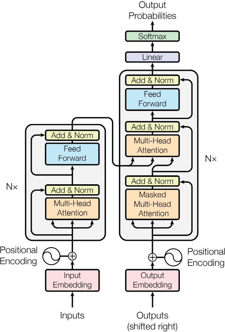
We have an input/prompt. We encode it and run it through N stacks of attention-feedforward as use it as input for the decoder to use.

We have a decoder. We put in the target output shifted right once as the input.

For example, we have an input [“what did the cat do <eos>”] and a target output ["<bos> the cat sat on the mat"].

At each output token, because we care about next-token prediction, we mask the future tokens that have not been output yet in the first attention step. This is essentially a triangular matrix.

For example, given an output target sequence:

             The   cat   sat   on   the
1 The         ✓     ✗     ✗    ✗    ✗
2 cat         ✓     ✓     ✗    ✗    ✗
3 sat         ✓     ✓     ✓    ✗    ✗
4 on          ✓     ✓     ✓    ✓    ✗
5 the         ✓     ✓     ✓    ✓    ✓

“cat” can only generate attention from “the cat”, and “on” can only generate attention from “the cat sat on”.

Then we do a cross-attention from the encoder. We feed the enriched encoder tensor into some learned projection (learnable weights) for K,V. The decoder tensor is fed into some learned projection for Q. Then it does the usual skip path and FFN steps to learn. This is done N times. The ‘stacking’ of modules is illustrated below.

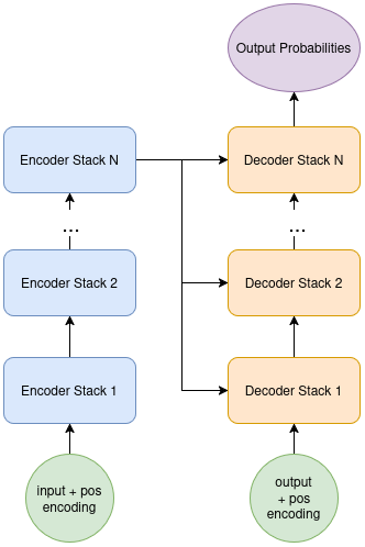
The very last step is to take the N-times enriched decoder tensor, put it through a final linear model with softmax to ouput the next token probabilities.

Phew.

This architecture was originally meant for translation, but has found its use for many other things. Modern LLMs are decoder-only and leave self-attention and FFNs as a stack.

What next?

We have effectively speedrun decades of research, and yet, we are generations behind what is SoTA today. And I am exhausted writing this primer so we will stop here.

For now, all of these primitives (neurons, memory, attention, etc) with all sort of permutations and modifications are the foundation of modern machine learning.

The next steps (as future work) are building more interesting things based on these primtives: Mixture of Experts, Hybrid Architectures, etc…