Gemini Probes Paper

⌛ 7 minutes read

This is a paper readalong for arxiv.org/pdf/2601.11516

AI safety is more important than ever, with models having increased capabilities.

One way to detect misuse of LLMs is with monitoring systems. If we can catch bad user inputs, then we can mitigate them. Gemini probes is a way to monitor such misuse.

WTF are probes?

Imagine a neuroscientist sticking a multimeter into your head to read your brain’s neurons to determine if you have evil thoughts. LLM probes are functionally the same.

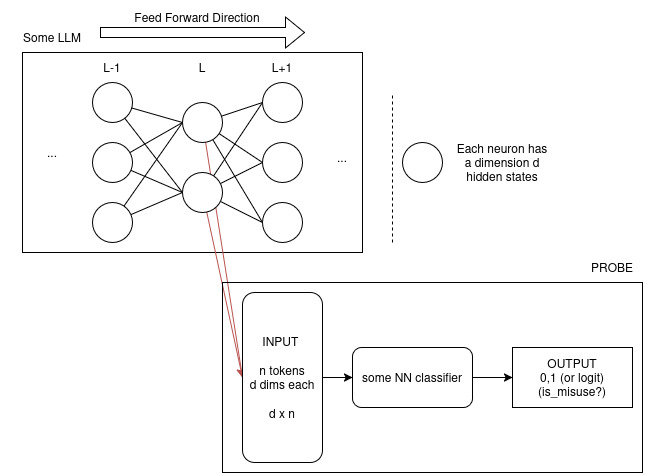
Neural Network layers have hidden activation states, so we read them and slap a trained classifier on it to predict if the activation state is evil or not.

Why does it work? The hand-wavy intuition is that “evil thoughts” (misuse patterns) have patterns in the voodoo activation states, and can be classified.

The Problem, and Experiments

The paper explores different probe architectures (including a diff between naiviely feeding inputs to an LLM itself to classify). We are interested in minimizing errors (missing out on evil prompts) while also keeping inference costs (how much compute do we spend) low.

The ’naiive¹’ solution, using LLM to classify the input, results in low-ish error and high cost. We want to see how different probes compare to these.

But there are issues. Although probes are cheap, they are “fragile to distribution shifts, particularly long-context inputs”. They don’t generalise. Training on long-context data is possible, but the authors claim that training costs rise by more than order of magnitude. Distribution shifts like jailbreaks, multi-turn data are also not really explored.

The paper is an effort to deal with these performance degredations, via novel probe architectures.

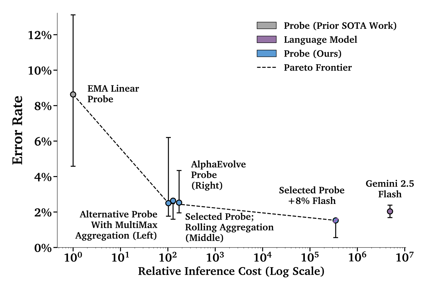
The rest of the paper explains this image and builds up to it.

Deeper Dive into Probe architecture

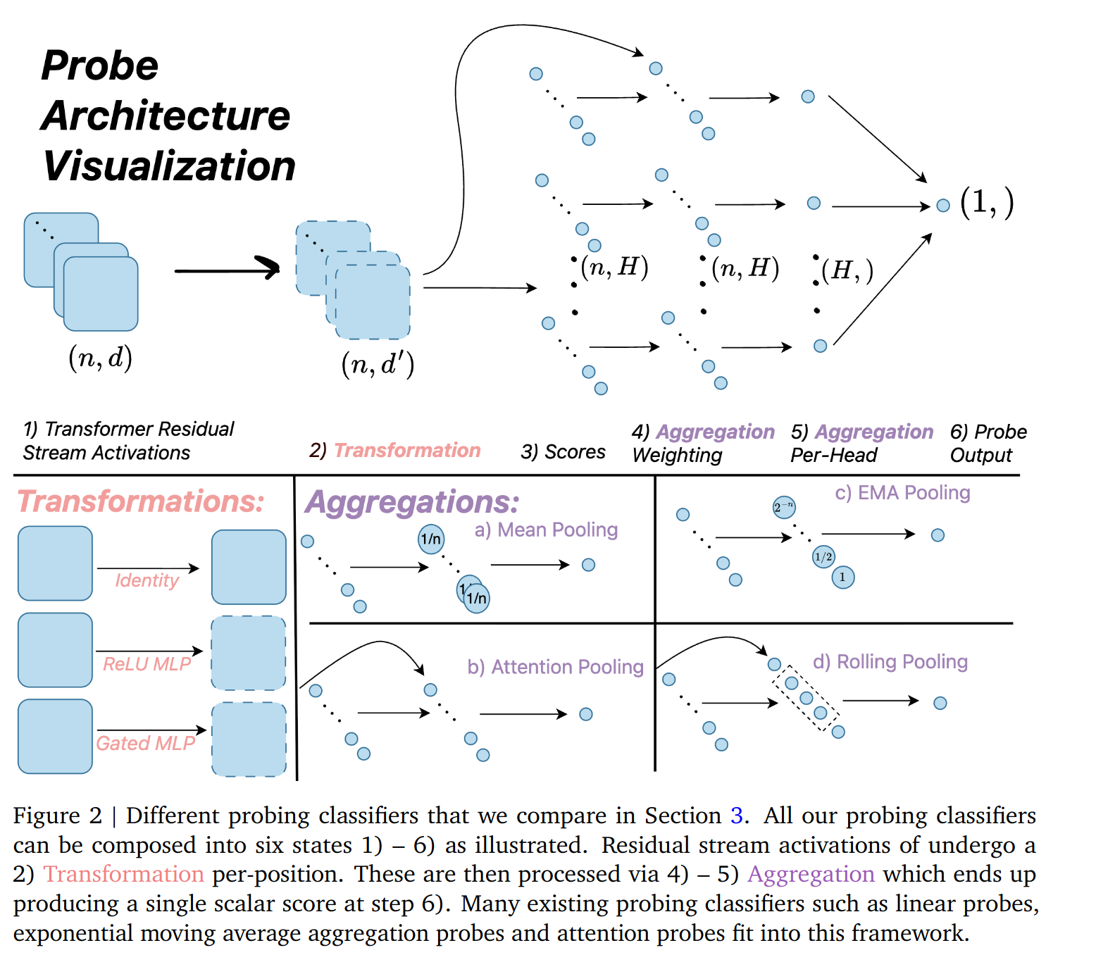
As below². The idea is that we leech off the (n,d) activation states (n=|tokens|, d=dims at the layer) from the (evil) LLM in question. We then do some math on the input to transform it from (n,d) to (1,).

The math involves a transformation step (n,d) -> (n,d’), and an aggregation step that transforms (n,d’) -> (1,).

The spicy sauce is in the specifics of the math. The traditional (already explored in literature when the paper was written) ways of processing it uses Mean, Attention, EMA, Rolling pooling.

The research question is - these traditional methods have flaws. Can we do better?

Traditional Probes

This section explains in ‘plainer english’ the diagram (fig 2) above. The ’traditional’ probes (relative to what this paper presents) make use of three forms of transformations.

The identify transformation does nothing to the original (n,d) input. d = d’.
The ReLU MLP transformation applies a learned non-linear map. d’ is arbitrary.
The gated MLP transformation applies another type of learned non-linear map. d’ is arbitrary.

Essentially, the transformations just adds some weights to the original input. This makes sense - perhaps some activation states in some dimension matters more than others.

Then, we need to aggregate the results. Aggregation takes the transformed input and then divides it into H heads. Each head undergoes some form of aggregation that has some math related to it (mean, EMA, attention are just math functions).

We eventually pool the heads as well to get a single scalar value. is_evil?

The gory math details are an exercise for the reader (read the paper!).

MultiMax Probes

The paper explores a bunch of ’novel’ architectures to deal with long-context generalization issues.

We start with multimax probes.

Multimax probes improve on attention probes. Attention probes use softmax. The issues with softmax is that it overtriggers on long contexts.

Multimax takes the highest scoring token per head rather than computing a weighted average. The effect is the the ’evil’ signal is not as diluted when ’evil’ content appears in a small part of a large context.

The following example is AI generated but I think illustrates how softmax dilutes important tokens well:

{begin_ai}

Per-token values v_j = vᵀ y_j. Token 3 carries the signal, and the probe attends to it with a moderate score (s_3 = 2, all others 0).

 0
 1
 2
 3
 4
 5
 6
 7
 8
 9
10
Short context, n = 5
v: 0, 0, 8, 0, 0
s: 0, 0, 2, 0, 0
Softmax: exp(s) = 1, 1, 7.39, 1, 1   Z = 11.39   α_3 = 0.649
         output = Σ α·v = 0.649 · 8 = 5.19
Max:     output = 8

Long context, n = 100 (same signal, 99 benign tokens with v = 0, s = 0)
Softmax: Z = 7.39 + 99 = 106.39      α_3 = 0.069
         output = 0.069 · 8 = 0.56
Max:     output = 8

{end_ai}

Max of Rolling Means Attention Probe

A mouthful to read, but descriptive.

Rolling means = take the average of every window (this should be obvious if you have image processing background).

Consider this (6,1) tensor.

The rolling mean takes the average.

0
1
2
3
window ending t=3: tokens 1-3 → (1+0+2)/3 = 1.00
window ending t=4: tokens 2-4 → (0+2+3)/3 = 1.67
window ending t=5: tokens 3-5 → (2+3+4)/3 = 3   ← max
window ending t=6: tokens 4-6 → (3+4+0)/3 = 2.33

The authors make the setup more complicated. Instead of a simple arithmetic mean, they use attention-weighted averages. First take the sum of each token and its corresponding attention weight in the window. Then, take the sum of all the attention weights. Divide the former over the latter. We get the ‘rolling attention weighted mean’ of the token.

An example would help. Take a window of size 3.

token   a_j   v_j
1       1     1
2       1     2
3       2     8
4       2     2
5       1     1

Then, the sum of $a_j * v_j$, sum of $a_j$, and the corresponding $\bar{v}_t$

token   sum(a*j)  sum(a_j)  v_t
3       19        4         4.75  <-- max of v_t
4       22        5         4.4
5       21        5         4.2

This is illustrative, but the real hardcore math & notation is left as an exercise to the reader again.

These 2 new aggregation formulations were then tested against LLM-only classifiers, traditional probes, and 2 other novel architectures proposed by AlphaEvolve (automated discovery).

Results & Limitations

Into the evaluation jungle! I’m going to gloss through alot of the science…

The gist is that AlphaEvolve’s MultiMax variation and the Max of Rolling Mean Attention Probes outperform the baseline linear probes. Compared to the naiive “use llm to solve everything” solution, the (brace for incoming word salad!) Max of Rolling Mean Attention Probe with MultiMax aggregation outperforms.

Nice! But across the different ‘distribution shifts’, no method dominates. This is an area for deeper improvement (by the algo nerds).

Cascading Classifiers

Also discussed was the idea of cascading classifiers. Probe first classifies each query. Uncertain queries are shuttled off (deferred) to an LLM to judge. This probably makes some sense in production systems.

Anyway, choosing an optimal deferral rate is not cleanly explained and a precise science. But deferral works in improving accuracy compared to just using probes or LLMs.

Final Thoughts

The math behind probes isn’t all that complicated. The technology is also quite interesting, and surprisingly this paper wasn’t too hard to follow. The gist can be chewed through in a few hours.

There’s also a discussion about using AlphaEvolve to automate research, and it’s genuinely interesting to read but I’m not going to distill it here for focus.

The takeaway is that probes are efficient, can be enhanced with augmentation, and the fight to ‘solve’ distribution shifts is always in progress.